TL;DR

How does it affect model performance?

Dropping unimportant columns should not decrease the model performance. By removing a bunch of columns we can get rid of the source of collinearity between the features. The importance that previously was split between the columns should only be reflected in the one left in the model. This makes the feature importance values more clear and reliable.

For example random forest has less columns to try making a split, so it has a slightly better chance to make a better decisions. Model should take less time to run.

The biggest gain comes in less variables that a modeler needs to understand and worry in a model.

Data pre-processing

There are few things to be done with the data before pluging them into the model.

• I need to handle missing data both in numeric and cardinal columns. In the numeric columns missing values are replaced with median with a recipe step step_medianimpute(). I add a dummy column for every numeric column that contains NAs using add_dummy_for_na_numeric() that I define myself. I replace NAs in character columns with “NA” string and threat missing values as a separate level.
• I make sure my cardinal variables enter the model as factors. I use recipe step_novel() to make sure model can handle unseen levels in the validation set.
• I add new features based on sale date column to help the model handle time better. New features are: elapsed number of days since 1 Jan 1970, day, week, month, year, day of week, day of year and indicators is year/quarter/month beginning/end and are added using proc_date().

add_dummy_for_na_numeric <- function(x){
  x %>%
    mutate_if(~any(is.na(.)) & is.numeric(.),
              .funs = list(na = ~if_else(is.na(.), 1, 0)))
}

proc_date <- function(data, var_name) {
  data %>%
    dplyr::mutate(
      elapsed = floor(unclass(as.POSIXct({{var_name}}))/86400),
      year = lubridate::year({{var_name}}),
      month = lubridate::month({{var_name}}),
      day = lubridate::day({{var_name}}),
      week = lubridate::week({{var_name}}),
      day_of_week = lubridate::wday({{var_name}}),
      day_of_year = lubridate::yday({{var_name}}),
      is_end_of_month = if_else({{var_name}} == (ceiling_date({{var_name}}, unit = "month") - 1), TRUE, FALSE),
      is_begining_of_month = if_else({{var_name}} == floor_date({{var_name}}, unit = "month"), TRUE, FALSE),
      is_end_of_quarter = if_else({{var_name}} == (ceiling_date({{var_name}}, unit = "quarter") - 1), TRUE, FALSE),
      is_begining_of_quarter = if_else({{var_name}} == floor_date({{var_name}}, unit = "quarter"), TRUE, FALSE),
      is_end_of_year = if_else({{var_name}} == (ceiling_date({{var_name}}, unit = "year") - 1), TRUE, FALSE),
      is_begining_of_year = if_else({{var_name}} == floor_date({{var_name}}, unit = "year"), TRUE, FALSE)
      
    )
    
}

Pre-process data by calling helper functions:

data_after_basic_preprocess <- data_raw %>%
  dplyr::mutate(
    saledate = lubridate::as_date(saledate, format = "%m/%d/%Y %H:%M")
    ) %>%
  arrange(saledate) %>% 
  proc_date(saledate) %>% 
  mutate_if(is_character, ~if_else(is.na(.), "NA", .)) %>% 
  add_dummy_for_na_numeric()

I take the log of SalePrice. Taking the log of the SalePrice makes the variable normally distributed and changes the relative distance between numbers.

data_step1 <- data_after_basic_preprocess %>%
  mutate(log_SalePrice = log(SalePrice),
         saledate = NULL,
         SalePrice = NULL)

Split data into training and validation set using initial_time_split() function. I keep 80% of data in the training set and 20% in the validation. initial_time_split() is called on data which is sorted based on saledate so I make sure validation set contains “future sales”. Taking a random sample would be cheating here, as we would use “future information” to predict the past.

data_step1_split <- initial_time_split(data = data_step1, prop = 0.80)

train_set <- training(data_step1_split)

valid_set <- testing(data_step1_split)

The rest of the pre-processing is done using recipes package:

• Replacing NAs in numeric columns with their median with step_medianimpute()
• Changing characters to factors with step_string2factor()

Additionally recipe() takes care of new levels in validation set using step_novel().

recipe_formula <-  recipe(log_SalePrice ~ ., data = data_step1_split)

recipe_steps <- recipe_formula %>%
  step_novel(all_nominal()) %>% 
  step_medianimpute(all_numeric()) %>%
  step_string2factor(all_nominal())

recipe_steps_on_training <- recipe_steps %>% 
  prep(train_set)

Now let’s juice and bake training and validation sets and split x and y for ranger model to avoid using formula.

train_set_preped <- recipe_steps_on_training %>%
  juice()

y_train <- train_set_preped$log_SalePrice
x_train <- train_set_preped %>% select(-log_SalePrice)


valid_set_preped <- recipe_steps_on_training %>%
  bake(valid_set)

x_valid <- valid_set_preped %>% select(-log_SalePrice)
y_valid <- valid_set_preped$log_SalePrice

Model building

I build random forest using ranger package. I’m not using randomForest, because it has very slow implementation in R. I limit the number of trees to speed the training process to 40.

To avoid over-fitting:

• use a subset of columns when building trees by setting mtry parameter to build less correlated trees,
• use a subset of rows when building trees by setting sample.fraction, can be used to build less correlated trees and speed up training,
• stop training the tree further when a leaf node has 3 or less samples. Numbers that usually works well 1, 3, 5, 10, 25.

Categorical variables enter the model as factors and ranger will treat them as ordered. This might seem controversial, but it has been shown by the one of the ranger authors Marvin Wrigth and Inke König that treating factors like that shouldn’t impact final result, but is computationally more efficient.

system.time(ranger_model_with_sampling <- ranger(x = x_train,
                       y = y_train,
                       num.trees = 40,
                       mtry = (ncol(x_train) / 2), 
                       seed = 1,
                       min.node.size = 3,
                       sample.fraction = 1,
                       respect.unordered.factors = "ignore"
                       ))

## Growing trees.. Progress: 23%. Estimated remaining time: 2 minutes, 21 seconds.
## Growing trees.. Progress: 53%. Estimated remaining time: 1 minute, 14 seconds.
## Growing trees.. Progress: 83%. Estimated remaining time: 25 seconds.

##    user  system elapsed 
## 552.498   0.789 142.328

ranger_predictions <- predict(ranger_model_with_sampling, x_valid)

rmse <- function(preds, y){
  sqrt(mean((preds - y)**2))
}
eval_model <- function(model, y, y_valid, model_predictions) {
  c(model$r.squared,
      rmse(model$predictions, y),
      rmse(model_predictions, y_valid)
  )
}

eval_model(
  ranger_model_with_sampling, y_train, y_valid, ranger_predictions$predictions)

## [1] 0.9106202 0.2062955 0.2664465

Model interpretation

Now when I have my random forest built I can try to understand it and look at variable importance plot. I use DALEX package and create ranger explainer. DALEX package provides tones of useful tools for understanding black box models.

explainer_ranger  <- explain(ranger_model_with_sampling,
                             data = x_train,
                             y = y_train)

## Preparation of a new explainer is initiated
##   -> model label       :  ranger  (  default  )
##   -> data              :  320900  rows  66  cols 
##   -> data              :  tibble converted into a data.frame 
##   -> target variable   :  320900  values 
##   -> predict function  :  yhat.ranger  will be used (  default  )
##   -> predicted values  :  numerical, min =  8.480695 , mean =  10.09761 , max =  11.84336  
##   -> model_info        :  package ranger , ver. 0.12.1 , task regression (  default  ) 
##   -> residual function :  difference between y and yhat (  default  )
##   -> residuals         :  numerical, min =  -1.185159 , mean =  -7.183829e-05 , max =  0.9795716  
##   A new explainer has been created! 

I use variable_importance() function from ingredients (DALEX family) package to calculate the variable importance. My loss function is RMSE. DALEX performs by default 10 permutation rounds. I will average the permutation results and inspect the plot for the best 30 features (for better plot readability). I drop _baseline_ from the plot. Baseline is the change in model performance when all variables are permuted.

var_importance <- variable_importance(explainer_ranger,
                                      loss = loss_root_mean_square,
                                      B = 10,
                                      type = "raw")

summarize_vi <- var_importance %>%
  group_by(variable) %>% 
  summarize(mean_dropout_loss = mean(dropout_loss), .groups = "drop") %>%
  arrange(-mean_dropout_loss) %>%
  mutate(variable = factor(variable, levels = variable))  

ggplot(data = summarize_vi[2:31,],
       aes(y = mean_dropout_loss, x = variable, group = 1)) +
  geom_line() +
  theme(axis.text.x = element_text(angle = 45, hjust = 1))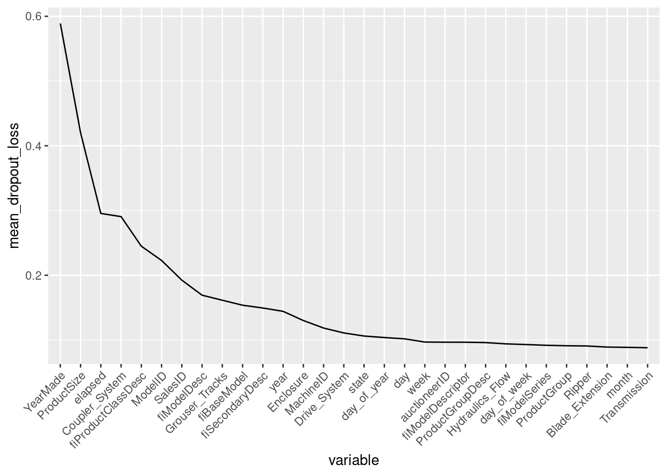

There are only few variables that my random forest cares about. YearMade is the most important one. So next I select the features before the curve flattens almost completely at around 0.1 mean dropout loss and build a model on the remaining features subset.

var_to_keep <-  summarize_vi %>%
  filter(mean_dropout_loss > 0.1 & variable != "_baseline_") %>% 
  select(variable)

x_after_var_importance <- x_train %>% select(var_to_keep$variable)

system.time(ranger_model_after_vi <- ranger(x = x_after_var_importance,
                       y = y_train,
                       num.trees = 40,
                       mtry = (ncol(x_after_var_importance) / 2),
                       seed = 1,
                       respect.unordered.factors = F,
                       min.node.size = 3,
                       sample.fraction = 1))

## Growing trees.. Progress: 63%. Estimated remaining time: 20 seconds.

##    user  system elapsed 
## 199.450   0.501  51.292

ranger_predictions_after_vi <- predict(ranger_model_after_vi,
                                       x_valid %>% select(var_to_keep$variable))

eval_model(
  ranger_model_after_vi, y_train, y_valid, ranger_predictions_after_vi$predictions)

## [1] 0.9089519 0.2082119 0.2692650

I end up with a simpler model with almost the same quality, differences in R^2 and RMSE are neglectable. I prefer to continue with model with less features which runs faster.

Let’s again look at variable importance plot and do more digging.

explainer_ranger_after_vi  <- explain(ranger_model_after_vi,
                                      data = x_after_var_importance,
                                      y = y_train)

## Preparation of a new explainer is initiated
##   -> model label       :  ranger  (  default  )
##   -> data              :  320900  rows  18  cols 
##   -> data              :  tibble converted into a data.frame 
##   -> target variable   :  320900  values 
##   -> predict function  :  yhat.ranger  will be used (  default  )
##   -> predicted values  :  numerical, min =  8.482757 , mean =  10.09765 , max =  11.84426  
##   -> model_info        :  package ranger , ver. 0.12.1 , task regression (  default  ) 
##   -> residual function :  difference between y and yhat (  default  )
##   -> residuals         :  numerical, min =  -1.201127 , mean =  -0.0001043412 , max =  0.9551131  
##   A new explainer has been created! 

var_importance_ranger_after_vi <- variable_importance(
  explainer_ranger_after_vi,
  loss_function = loss_root_mean_square,
  B = 10,
  type = "raw")

plot(var_importance_ranger_after_vi)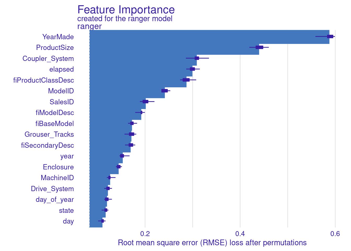

YearMade is the most important feature for my model. It would be interesting to learn more about this variable. Second thing that stands out is how important are SalesID and MachineId. I expect these are unique identifiers so it’s strange they are so important. So it’s another thing worth looking into.

ggplot(data_step1, aes(x = YearMade)) + 
  geom_histogram(binwidth = 10)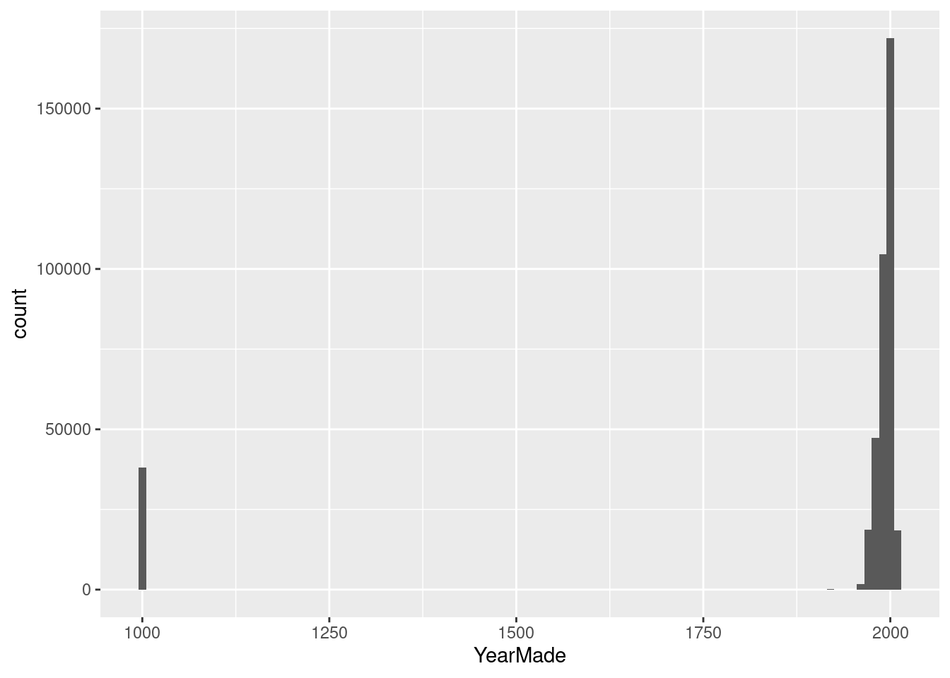

data_step1 %>% group_by(YearMade) %>% count()

## # A tibble: 72 x 2
## # Groups:   YearMade [72]
##    YearMade     n
##       <dbl> <int>
##  1     1000 38185
##  2     1919   127
##  3     1920    17
##  4     1937     1
##  5     1942     1
##  6     1947     1
##  7     1948     3
##  8     1949     1
##  9     1950     8
## 10     1951     7
## # … with 62 more rows

After plotting YearMade distribution I can see that sth weird is happening. There is 38185 entries with YearMade 1000. This is not possible, so I remove this data and use the sales after the War ended.

data_step1$SalesID %>% n_distinct()

## [1] 401125

data_step1$MachineID %>% n_distinct()

## [1] 341027

data_step1 %>%
  filter(MachineID == 2283592)

## # A tibble: 26 x 67
##    SalesID MachineID ModelID datasource auctioneerID YearMade MachineHoursCur…
##      <dbl>     <dbl>   <dbl>      <dbl>        <dbl>    <dbl>            <dbl>
##  1 4319298   2283592    4579        172            1     2002             3802
##  2 4319348   2283592    4579        172            1     2006             1764
##  3 4319347   2283592    4579        172            1     2006              831
##  4 4319295   2283592    4579        172            1     2005                0
##  5 4319353   2283592    4579        172            1     2004             3405
##  6 4319296   2283592    4579        172            1     2004             3405
##  7 4319355   2283592    4579        172            1     2005             2201
##  8 4319294   2283592    4579        172            1     2005             2201
##  9 4319350   2283592    4579        172            1     2005             2050
## 10 4319335   2283592    4579        172            1     2005             2050
## # … with 16 more rows, and 60 more variables: UsageBand <chr>,
## #   fiModelDesc <chr>, fiBaseModel <chr>, fiSecondaryDesc <chr>,
## #   fiModelSeries <chr>, fiModelDescriptor <chr>, ProductSize <chr>,
## #   fiProductClassDesc <chr>, state <chr>, ProductGroup <chr>,
## #   ProductGroupDesc <chr>, Drive_System <chr>, Enclosure <chr>, Forks <chr>,
## #   Pad_Type <chr>, Ride_Control <chr>, Stick <chr>, Transmission <chr>,
## #   Turbocharged <chr>, Blade_Extension <chr>, Blade_Width <chr>,
## #   Enclosure_Type <chr>, Engine_Horsepower <chr>, Hydraulics <chr>,
## #   Pushblock <chr>, Ripper <chr>, Scarifier <chr>, Tip_Control <chr>,
## #   Tire_Size <chr>, Coupler <chr>, Coupler_System <chr>, Grouser_Tracks <chr>,
## #   Hydraulics_Flow <chr>, Track_Type <chr>, Undercarriage_Pad_Width <chr>,
## #   Stick_Length <chr>, Thumb <chr>, Pattern_Changer <chr>, Grouser_Type <chr>,
## #   Backhoe_Mounting <chr>, Blade_Type <chr>, Travel_Controls <chr>,
## #   Differential_Type <chr>, Steering_Controls <chr>, elapsed <dbl>,
## #   year <dbl>, month <dbl>, day <int>, week <dbl>, day_of_week <dbl>,
## #   day_of_year <dbl>, is_end_of_month <lgl>, is_begining_of_month <lgl>,
## #   is_end_of_quarter <lgl>, is_begining_of_quarter <lgl>,
## #   is_end_of_year <lgl>, is_begining_of_year <lgl>, auctioneerID_na <dbl>,
## #   MachineHoursCurrentMeter_na <dbl>, log_SalePrice <dbl>

SalesID is a unique identifier that sorts sales from the oldest to the newest. Kaggle’s description says MachineID is unique machine identifier and that machine can be sold multiple times. I expect that RF model could be overfitting on these columns so I remove them from the dataset and see how it impacts the model.

x_train <- x_train %>%
  mutate(YearMade = if_else(YearMade >= 1950, YearMade, 1950)) %>%
  select(var_to_keep$variable) %>%
  select(-c(SalesID, MachineID))

x_valid <- x_valid %>%
  mutate(YearMade = if_else(YearMade >= 1950, YearMade, 1950)) %>%
  select(var_to_keep$variable) %>%
  select(-c(SalesID, MachineID))

system.time(ranger_model_after_vi_data_clean <- ranger(x = x_train,
                       y = y_train,
                       num.trees = 40,
                       mtry = (ncol(x_train) / 2),
                       seed = 1,
                       min.node.size = 3,
                       sample.fraction = 1))

## Growing trees.. Progress: 83%. Estimated remaining time: 6 seconds.

##    user  system elapsed 
## 148.966   0.442  38.453

ranger_predictions_after_vi_clean <- predict(ranger_model_after_vi_data_clean,
                                       x_valid)

eval_model(
  ranger_model_after_vi_data_clean, y_train, y_valid, ranger_predictions_after_vi_clean$predictions)

## [1] 0.9104619 0.2064781 0.2667099

It seems cleaning YearMade and dropping IDs improved the model just a bit.